21 Mar 2017: Lab 4: Trajectories

Lab 4: Trajectories

Joel Cook

Nina Song

Lab performed on March 14, 2017

In this lab, we were attempting to predict the trajectory of an object. 

Introduction: Through experimentation, kinematics, and projectile motion, we are able to calculate the speed of an object rolling off of a track and predict where the object will land when the conditions are changed.

Apparatus and Procedure: In this lab, we used two pieces of aluminum v-channel to form a track for a steel ball to roll on, as pictured below. One end of one of the pieces was elevated to increase the velocity of the ball consistently for all five trials.

A piece of paper was taped to the floor with a carbon paper taped to the top at approximately the distance we expected the ball to fall to. This was done in order to record the exact position that the ball strikes the floor each time. We can then measure the distance from the end of the track to the where the ball strikes (ΔX) and the distance from the end of the track to the floor (ΔY). 

From the recorded distances we are able to calculate the speed of the ball as it leaves the track, as shown below. The uncertainty in the measurements for distance are shown after the value measured.

As shown in the calculations above, by using the kinematics equations for displacement, vertically and horizontally, we are able to substitute for time and solve for initial speed, or the speed of the ball as it leaves the track. 

In the second part of the lab, we leaned a board against the table in the path of the falling ball and measured the angle. 

We measured the angle as 49.0 +/- 0.5 degrees. As shown below, knowing initial speed and the angle we can derive an expression for how far down the board the ball will strike (d).

As shown, we calculated that the ball would strike the board 0.939 meters down the board. We taped a piece of paper and carbon paper, as before, to the board where the ball would land. We performed five trials and measured that the ball landed 0.915 +/- 0.005 meters down the board.

Conclusion: We were able to predict the location that the ball would strike the board with good accuracy. This calculation would have been more accurate but there was uncertainty in our measurements. The uncertainty in our displacement measurements and angle measurements reduce the accuracy with which we can predict the striking of the ball. In addition, errors may have existed in our lab that went unnoticed. The track may have moved without noticing and the board may have moved when struck each time by the ball.

The propagated uncertainty was calculated in this lab and is shown below. The uncertainty in the final calculation comes from the uncertainty in measuring horizontal displacement, vertical displacement, and angle of the board. First, dVo was calculated from the uncertainty in x and y. The result of this was used to calculate the dd using the uncertainty in Vo and the uncertainty in the angle. 

The calculation for the distance down the board that the ball would strike (d) is shown as 0.939 +/- 0.051m. Our measured distance of 0.915 meters was off by 0.024 meters, which is well within the uncertainty calculated in the propagated uncertainty above. Therefore, our lab was successful. 

13 Mar 2017: Lab 4: Modeling the Fall of an Object with Air Resistance

Lab 4: Modeling the Fall of an Object with Air Resistance

Joel Cook

Nina Song

Lab performed March 13, 2017

In this experiment, we are attempting to develop a model for calculating the air resistance and terminal speed of an object.

Introduction: The air resistance an object experiences depends on the speed, shape, and mass of an object. By using video capture, we can analyze the speed, acceleration, distance, and time an object travels. By analyzing coffee filters being dropped, we are able to calculate the terminal velocity of the coffee filter. In the second part of this experiment, we use Microsoft Excel to numerically determine the terminal velocity of coffee filters and compare the results against the video capture to determine if the model created is acceptable. We expect that the air resistance can be calculated using the equation
F=kv^n, where F is air resistance force, k is a constant for shape and area of the object, and v is speed. 

Apparatus/Procedure: In this lab, we used a laptop computer and logger pro to capture and analyze the video of coffee filters being dropped. We captured video of one filter being dropped, two filters together being dropped, and repeated for a total of five filters dropped together. The filters were stacked together to keep the shape of the object the same but change the mass for each trial. The videos were analyzed to plot the position of the filter versus time. A linear fit of the last portion of the data shows the terminal velocity of the coffee filter, which is the slope of the line through the points. A graph of Air Resistance Force versus speed was created showing one through five filters. A power fit of this data generates a model for calculating the Net Force on an object. 

For the second part of the experiment, we used Microsoft Excel to numerically analyze the data using the model created in the first part of the lab. The spreadsheet uses time, speed, net force, acceleration, mass of the object, and the equation determined part one, to calculate the terminal velocity. We are able to compare the values observed in experiment to the values determined from the model to determine how good our model is. In the spreadsheet, time used was increments of 0.05 seconds, Net Force is mass times acceleration minus Air Resistance Force (k*v^n), acceleration starts at g and is Net Force divided by mass, change in speed is acceleration calculated times time increment, and speed is previous speed plus the calculated change in speed. By adding rows to the spreadsheet, we can see the point when velocity stops increasing and acceleration is zero. This velocity is the terminal velocity, or the highest velocity the object can reach in free fall.

Data: 

The photo below shows the data generated from the video capture for one coffee filter dropped. The terminal velocity shown by the slope of the linear fit of the data is 1.263 m/s.

The photo below shows the data generated from the video capture for two coffee filters dropped. The terminal velocity shown by the slope of the linear fit of the data is 1.679 m/s.

The photo below shows the data generated from the video capture for three coffee filters dropped. The terminal velocity shown by the slope of the linear fit of the data is 2.106 m/s.

The photo below shows the data generated from the video capture for four coffee filters dropped. The terminal velocity shown by the slope of the linear fit of the data is 2.508 m/s.

The photo below shows the data generated from the video capture for five coffee filters dropped. The terminal velocity shown by the slope of the linear fit of the data is 2.728 m/s.

The photo below shows the data generated by plotting the terminal velocities versus mass. A power fit of the curve is shown.

The equation for air resistance is now F=kv^n is now F = 0.0005989 * v ^ 1.958
The uncertainty in k is +/- 0.00005879 (N*s/m) and the uncertainty in n is +/- 0.1086.

For the second portion of the lab, we determined the terminal velocity based on numerical analysis using Microsoft Excel. The photo below shows the result for terminal velocity of one coffee filter being dropped. The terminal velocity was calculated as 1.2115 m/s.

The photo below shows the result for terminal velocity of two coffee filters being dropped. The terminal velocity was calculated as 1.7261 m/s.

The photo below shows the result for terminal velocity of three coffee filters being dropped. The terminal velocity was calculated as 2.1213 m/s.

The photo below shows the result for terminal velocity of four coffee filters being dropped. The terminal velocity was calculated as 2.4593 m/s.

The photo below shows the result for terminal velocity of five coffee filters being dropped. The terminal velocity was calculated as 2.7562 m/s.

The table below summarizes the results for the video analysis versus the numerical analysis:

# of Filters	Mass of Filters (kg)	Terminal Velocity from Video Analysis (m/s)	Terminal Velocity from Numerical Analysis (m/s)	Difference
1	8.72E-04	1.263	1.2115	0.0515
2	1.74E-03	1.679	1.7261	-0.0471
3	2.62E-03	2.106	2.1213	-0.0153
4	3.49E-03	2.508	2.4593	0.0487
5	4.36E-03	2.728	2.7562	-0.0282

For all cases, the value for terminal velocity calculated in Microsoft excel was within 0.1 m/s of the value calculated from the video analysis method.

Conclusion: Our model we created for determining air resistance and modeling terminal velocity end up being very very accurate but there are variables in the lab that are difficult, or impossible, to control. When filming the coffee filters, the lens of the camera is turning a cone shaped image into a flat image which will shorten the distances at the edges of the image; therefore the most accurate velocities are when the coffee filter was in the center of the image. It is not possible to account for this in the data. In addition, the video analysis requires clicking on a slightly blurry coffee filter that was difficult to see and impossible to click identically for each frame of each video. Patience and persistence helped to make the video analysis as accurate as possible but uncertainty in the data exists for this portion. Finally, when scaling the video during analysis, there is uncertainty in the accuracy of properly selecting the right distance for the scale. These possible uncertainties were considered and mitigated as much as possible by careful analysis of the videos. 

8 Mar 2017: Lab 3: Non-Constant Acceleration Problem

Lab 3: Non-Constant Acceleration Problem:

Rocket-Powered Elephant

Joel Cook

Nina Song

Lab performed March 8, 2016

In this lab, we have been given a physics problem in which an elephant on skates rolls down a hill with a rocket on his back pointing backwards. At the bottom of the hill the rocket fires and we are tasked with finding how far the elephant will travel before it stops and how long it will take. We are using Microsoft Excel to perform the calculations.

Introduction: Performing the calculations requested in this lab involve using calculus in order to calculate distance travelled and time with an acceleration that is changing. The professor has performed the calculus and provided the solution to the problem. The intent of the lab is to use Microsoft Excel to perform the calculations quickly and efficiently to reach the same solutions. 

Procedure: A computer with Microsoft Excel was used to perform the calculations. The initial conditions and formulas were input into the spreadsheet and the computer generates the results. We then reduced the time interval incrementally to find a more precise answer to the question. In the last part of the lab, we changed the initial conditions in the problem and found a different set of solutions. The results are shown below:

The first set of data shows the result for a time interval of 1 second. The distance traveled is shown as 247.9 meters in 20 seconds. The second set shows the result for a time interval of 0.1 seconds. The distance traveled is shown as 248.6 meters in 19.7 seconds. The third set shows the result for a time interval of 0.05 seconds. The distance traveled is shown as 248.66 meters in 19.70 seconds.

Questions: 
1. The solution that was provided analytically is 248.7 meters in 19.69075 seconds. The answer we achieved numerically is 248.66 meters in 19.70 seconds. Essentially the same answer.

2. We had the analytical solution to compare our value against. We were able to change the time interval to achieve a similar accuracy to the analytical solution. To determine the time interval is small enough in the numerical approach with the analytical approach to compare to, we can change the time interval in the spreadsheet until the number in the decimal place we are interested in (i.e. hundredths place) stops changing. It is not necessary to achieve a precision that takes the answer to 5 or 10 decimal places.

3. The last set of data pictured above shows the results for a different set of initial conditions. The distance travelled would be 163.99 meters in 12.95 seconds before the elephant stops.

Conclusion: In this experiment, we showed that Microsoft Excel can be used to perform calculations for distance travelled and time with a changing acceleration and achieve the same solution one would arrive at using calculus and an analytical method. The experiment was a resounding success.

6 Mar 2017: Lab 2: Calculating Acceleration due to Gravity

Lab 2:

Calculating Acceleration due to Gravity

Joel Cook

Nina Song

Angel Sanabvia

Lab performed March 2, 2017

In this experiment, we are calculating acceleration due to gravity (g) by using a free fall apparatus and Microsoft Excel.

Introduction: In this lab, we have an apparatus that creates a tape marked every 1/60th of a second. By measuring the distance between the marks on the tape and the time between marks, we are able to calculate acceleration due to gravity. Microsoft Excel, a computer spreadsheet program, is used to perform the calculations and graph the results. In addition, Excel was used to calculate the uncertainty in the data.

Part 1: Calculating g

Procedure: The apparatus pictured below was used to generate the tape with the marks for measuring. The apparatus has a magnet at the top holding a wooden cylinder with a metal ring around the cylinder. A long tape is secured to the apparatus. The cylinder is dropped between two wires and a spark is generated every 1/60th of a second. The metal ring of the cylinder transmits the spark to the tape as it falls making a mark every time the spark is generated. 

The tape was attached to the lab table and the distance between the marks were measured and recorded. A picture of the tape is shown below.

The data was recorded on a spreadsheet to facilitate quickly calculating the mid-interval times and speeds. A graph of the data was generated for mid-interval time vs. speed. A linear fit of the points shows the slope of the line drawn between the points and the slope represents the acceleration. In this case, the acceleration is due to gravity.

After all lab groups were finished calculating acceleration due to gravity, the data was collected on another spreadsheet to analyze the class data for average g calculated, deviation, and the root-mean-square. 

Data and Graphs: The image below shows the data gathered by our lab group.

The columns are labeled to show what the numbers below represent. Formulas were used to quickly calculate the information. TIME is 1/60th of a second for each interval, DISTANCE was measured on the tape in cm, ΔX is the difference between consecutive distances, MID-INTERVAL TIME is each time + 1/120th of a second for the middle of the interval, and MID-INTERVAL SPEED is the ΔDISTANCE/ΔTIME for each interval. A graph was generated from the data calculated that shows the mid-interval speed vs. time.

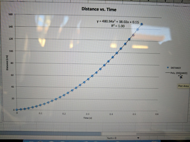
A graph of distance vs. time was created from the data gathered and shown below.

Questions: 

1. For the data presented the value of the mid-interval speed is equal to the average velocity over the same time interval:

Average velocity = ΔX/ΔT = (1.9 - 0.9)/(3/60 - 2/60) = 60 cm/s

Mid-interval speed = ΔX/1/60 = (1.9 - 0.9)/(1/60) = 60 cm/s

2. A linear fit of the data shows a slope of 963.58. This slope of a graph of speed vs. time is the acceleration, in this case acceleration due to gravity in cm/s^2. The calculated g for our group was 9.63 m/s^2. The accepted value for g is 9.8 m/s^2. The value calculated of 9.63 m/s^2 is lower than the accepted value of 9.8 m/s^2 by 0.17 m/s^2.

3. A power fit of the second graph shows a value of 480.94 as the first coefficient. The derivative of distance vs. time gives the equation for speed vs. time with the slope of this line being acceleration. The derivative of this equation gives a linear equation with a value of approximately 962 or 9.62 m/s^2 for acceleration due to gravity. The value calculated of 9.62 m/s^2 is lower than the accepted value of 9.8 m/s^2 by 0.18 m/s^2.

Part 2: Errors and Uncertainty

For the second part of this lab we gathered the class data for acceleration due to gravity and developed the following table:

We calculated the average for g as 962.852 cm/s^2. Next we calculated the root-mean-square to get a standard deviation of 10.0. The class, as a whole, calculated g to be 9.62 +/- 0.10 m/s^2 with 68% certainty (1 standard deviation) and 9.62 +/- 0.20 m/s^2 with 95% certainty (2 standard deviations). since the accepted value for g is 9.8 m/s^2, the class average was consistently below that value but the average value is within 2 standard deviations of the accepted value.

Questions:

1. The pattern in our values of g were that most of the values were less than the accepted value of g.

2. Our group also calculated g at below the accepted value, but within two standard deviations of the accepted value of 9.8 m/s^2.

3.  The pattern for calculated values of g was that most of the groups calculated g at less than the accepted value.

4. Our value of g was very close to the class average. A systematic error that may exist in this experiment are the possibility that the cylinder contacted the wires or tape of the apparatus causing friction and affecting acceleration. A random error that could exist would be the possibility of measuring some of the marks inaccurately with the meter stick. 

5. The objective of this portion of the lab is to explore uncertainty in our experiments and outcomes and discuss calculating the numeric value of this uncertainty to better understand our results. Understanding uncertainty helps to identify the accuracy of the experiment and the results and to identify portions of the experiment or tools that could be improved to increase the accuracy of the outcomes. The key ideas were calculating the average of a set of data, calculating the standard deviation through the root-mean-square method, and explaining errors that may exist in the experiment.

Conclusion: In summation, although our calculation for the acceleration due to gravity for this lab was close to the class average, it was not very close to the actual value of g. Although our value was below the accepted value of g, the importance of the experiment was not in confirming the value of g, but rather in exploring tools to analyze results and determine the accuracy of data sets. 

6 Mar 2017: Lab 6: Propagated Uncertainty in Measurements

Lab 6:

Propagated Uncertainty in Measurements

Joel Cook

Nina Song

Lab performed March 6, 2017

Introduction: In this lab we are practicing calculating the propagation of uncertainty in measurements by calculating the density of two cylinders and the uncertainty in the values.

Procedure: Calipers were used to measure the height and diameter of two cylinders. A digital scale was used to measure the mass of the cylinders. The height, diameter, and mass are used to then calculate the density. 

Data and Calculations:

	Mass (g)	Height (cm)	Diameter (cm)
Cylinder 1	69.4	3.42	1.88
Cylinder 2	27.6	5.03	1.58

ρ=    m   =      m    

           V       π (D/2)²h

Density of cylinder 1:

ρ=   69.4

         π(1.88/2)² *3.42

=7.30g/cm^3

Density of cylinder 2:

ρ=   27.6 

         π(1.58/2)² *5.03

=2.80g/cm^3

Calculating propagated uncertainty:

Density of cylinder 1 is 7.30 +/- 0.08 g/cm^3 (Accepted density of zinc is 7.13 g/cm^3)

Density of cylinder 2 is 2.80 +/- 0.04 g/cm^3 (Accepted density of aluminum is 2.70 g/cm^3)

Conclusion: The density we calculated for each cylinder was acceptably close to the accepted densities of each material, based on the conditions of the experiment. Uncertainty exists in the experiment in both the measurements taken, through accuracy of tools used, and in the purity of the samples used. Based on these uncertainties, the results of the lab are acceptable.